XCSAO: A Radial Velocity Package for the IRAF Environment

Michael J. Kurtz, Douglas J. Mink, William F. Wyatt, Daniel G. Fabricant, and Guillermo Torres
Harvard-Smithsonian Center for Astrophysics, Cambridge, MA 02138

Gerard A. Kriss
Department of Physics and Astronomy, Johns Hopkins University, Baltimore, MD 21218

John L. Tonry
Department of Physics, MIT, Cambridge, MA 02139

in Astronomical Data Analysis Software and Systems I, ASP Conf. Ser., Vol. 25, eds. D.M. Worrall, C. Biemesderfer, and J. Barnes, p. 432-438

Abstract

XCSAO is a software package for obtaining radial velocities of stars and galaxies from optical spectra using the cross-correlation method. It has been written to work within the IRAF environment, and is compatible with other packages being developed at SAO for optical spectra. We discuss the individual components of the package in terms of the decisions required to set up the package for a new instrument/observing program. Using artificial spectra we show the procedures necessary to optimize the set up parameters, and demonstrate the robustness of the package when applied to spectra from both stars and galaxies.

Keywords Data Analysis, Spectra, Radial Velocities, Redshifts

Introduction

During the decade of the 1980s all radial velocities produced at SAO, both stellar and extra-galactic, were reduced using a suite of FORTH routines on NOVA computers written by John Tonry (Tonry and Davis 1979) and maintained and extended by Bill Wyatt (Tonry and Wyatt 1988). Moving our reductions onto modern computers in the IRAF (Tody 1986) environment required a total rewritting of the code; this has resulted in the RVSAO package, the main parts of which are XCSAO, for cross-correlation velocities, and EMSAO for emission line velocities.

Copies of the source and IRAF installation scripts can be obtained by anonymous FTP at ftp://cfa-ftp.harvard.edu/pub/iraf/rvsao.tar.Z. A Readme file can be found in the same directory. XCSAO has been extensively tested on Decstations and Sparcstations and is expected to experience no major changes. EMSAO is still undergoing substantial revision. Both tasks have been in production use at SAO for the past year, and are currently in production use by several large redshift and radial velocity programs worldwide.

XCSAO has its origins in the XCOR program written by Gerry Kriss, as well as the FORTH code, and a FORTRAN rendition of it by Tonry. Eventually we included the continuum estimation methods from Mike Fitzpatrick's FXCOR. Our code was written and is being maintained by Doug Mink.

This paper presents a very brief overview of the capabilities of XCSAO, and some of the testing procedures we have developed for it. An extensive description of the program is in preparation for PASP (Kurtz, et al. 1992).

Elements of XCSAO

The following subsections describe briefly the elements of XCSAO in the order in which they occur in the code. We indicate those elements which we believe should receive critical attention when setting up XCSAO for a new instrument.

Input Formats

XCSAO takes lists of 1-dimensional wavelength calibrated spectra in the standard format used by the ONEDSPEC task in the NOAO package. Spectra may be either log or linear lamda binned. Two lists are required, one for the unknowns and one for the templates; each unknown will be compared separately with each template. Figure I shows the parameter file for XCSAO.

Figure I: Parameter File for XCSAO.

Rebinning

Spectra are rebinned into the specified number of log wavelength bins (NCOLS) so that there is the maximum possible overlap between the unknown and the template in the rest frame. This is achieved by iterating on the radial velocity a total of NZPASS times; in addition the user can choose an initial guess CZGUESS by setting CZINIT=yes. The error in the estimate of radial velocity can often be halved on the second pass.

Note that this binning suggests that it is worthwhile to have the template cover the broadest wavelength range possible, at a dispersion equal or better than the unknown's, the rebinning will then choose the proper wavelength region for maximal overlap, with the resolution determined by the unknown. We find that it is in all cases better to rebin to the next larger power of two than the number of actual pixels, rather than the next smaller.

Apodization

The spectra are apodized by a cosine bell over a specified percentage of its extent. The size of the apodized region should be kept as small as possible while still preventing ringing in the fourier transform. We have found 5\%\ is satisfactory for most spectra, but this should be set for each new instrument following some testing.

Continuum and Emission Line Suppression

The continuum is subtracted from each spectrum after being calculated by routines derived from the ICFIT task, and only slightly modified from their implementation in the FXCOR task in the RV0 package. There are a large number of possibilities here, different observing programs require different settings. This is the area which we believe deserves the most experimentation when setting up a reduction.

If EMCHOP=yes XCSAO will remove emission lines and replace them with the value of the continuum before performing the cross corelation. The emission lines are found using ICFIT, with parameters settable as for the continuum supression; the method for finding emission lines here is similar to that used in the sister task EMSAO. Removing emission lines is critical to finding absorption line redshifts from galaxies with emission lines, if the spectrum is too noisy for the emission line removal, or if it has sharp spurious absorption features from poor sky subtraction we recommend that the offending regions be exised by hand, using SPLOT.

Fourier Filtering

Before correlating the unknown with the template each is put through a bandpass filter in the fourier domain (unless TEMPFIL=yes, then the template is considered to have already been filtered). We have done a number of experiments with the fourier filter, some of the main results are:

1. The type of ramp used in the bandpass filter is not important (assuming it is a reasonable choice, a step function is not reasonable). We have therefore removed all the options for filter type from XCSAO, and use just a cosine bell.
2. The exact choice of the high pass roll-off is unimportant. in so far as it does not impinge on the main data region.
3. The exact choice of the low pass roll-on is critical to the reduction, it should be chosen with great care. This also effects the relation of the r statistic with the actual error, see below.
4. Use of a frequency weighting scheme which can be shown in the limit of infinitly wide spectra to produce the maximum likelihood estimation for the lag (radial velocity) (e.g. Hassab and Boucher, 1979) is not an effective technique for spectra similar to ours.

Cross Correlation

The normal fourier cross correlation, the transform of one spectrum times the conjugate of the transform of the other, is performed.

Peak Fitting

The user can set the function to use to fit the peak with PKMODE, normally this makes no significant difference in the velocity. The user also sets the fraction of the peak height to fit the function to with PKFRAC, .5 is the default choice. Because the spectrum is quantized in pixels while the fractional power point to fit to is not we perform two fits, one two pixels wider than the other, and report the weighted mean as the result of the fit.

Error Calculation

Following Tonry and Davis(1979) we calculate an error as a function of their r statistic. It can be shown analytically that for sinusoidal noise with a half width of the sinusoid equal to the halfwidth of the correlation peak that the mean error in the estimation of the peak of the correlation function is

error = (3w)/(8(1+r))

where w is the FWHM of the correlation peak, and r is the ratio of the correlation peak height to the amplitude of the antisymmetric noise.

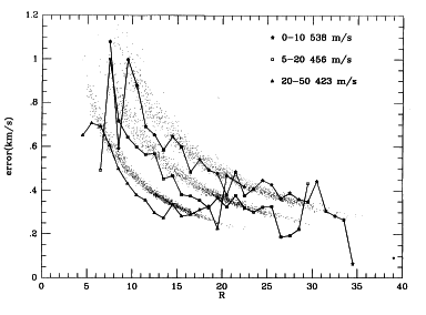
For large observing programs a better error estimate may be obtained. The coefficient 3/8 w is for many situations a constant, and may be estimated by taking the mean of a number of measures. The error estimate then becomes a constant divided by (1 + r). This is not in all cases possible, for example when the low pass fourier roll-on is changed the relation of r with error changes. 3/8 w tracks this properly. Figure II shows the calculated errors (dots) versus the actual mean errors (solid lines) as a function of the r statistic for three different low-pass filters; note that the calculated errors do track the actual errors, but that the relation of r with error changes.

Individual error estimates (dots) versus actual mean errors (solid lines) for 1200 synthetic echelle spectra. The three sets are for three different fourier filter roll-on points; the filter parameters, and the mean errors for each filter are shown on the figure.

Output Formats

While XCSAO may be run totally as a batch proceedure, it may also be run in an interactive mode. Intermediate stages in the reduction may be plotted, and the correlation peak to chose may be specified. At the conclusion of a reduction one may choose to redo the reduction interactively, to view a plot of the main absorption lines, to edit the emission lines, to remove spectral regions, ....

Primary output plot from XCSAO

Output plot showing absorption lines labeled

Figure III shows the standard final plot, and Figure IV shows an absorption line plot, both for a galaxy spectrum observed by M. Ramella with the ESO 1.5m telescope.

Testing

We have tested XCSAO with synthetic spectra created to have a specified number of counts sampled from a parent distribution, which is a template spectrum. For tests of echelle spectra we used Kurucz models for the templates, for tests of galaxy spectra we used high S/N observations. Note that we can know the true radial velocity difference between the unknowns and the templates either exactly in the case of models, or where the template spectrum was exactly the one used to create the synthetic spectra, or with very high accuaracy, as when the radial velocity template is different from the template used to create the synthetic spectra.

The data used to create Figure II were 1200 synthetic spectra created from a Kurucz model of a 5500K dwarf, and having between 5000 and 30,000 total counts. The template used for cross correlation was exactly the same template as was used to create the synthetic spectra. A complete description of the testing procedures will be found in Kurtz, et al. (1992).

Acknowledgments

Steve Levine and John Morse made important contributions to the development of the code. Dave Latham, Alejandra Milone, Susan Tokaraz, and John Huchra have contributed mightily of their expertise. Much of the IRAF code we have used was written by Mike Fitzpatrick and Frank Valdes.

References

Hassab, J.C. and Boucher, R.E. 1979, IEEE Trans. Acoust. Speech Signal Process., ASSP-27, 922

Kurtz, M.J., Mink, D.J., Wyatt, W.F., Fabricant, D.G., Torres, G., Kriss, G.A., and Tonry, J.L. 1992, Pub. Astron. Soc. Pacific, to be submitted

Tody, D. 1986, in Instrumentation in Astronomy VI, ed. D.L. Crawford, Proc. SPIE 627, 733

Tonry, J.L. and Davis, M. 1979, A Survey of Galaxy Redshifts I. Data Reduction, Astron. J., 84, 1511 [abstract] [full text]

Tonry, J.L. and Wyatt, W.F. 1988, CFA Z-Machine Data Analysis Software, Cambridge: Smithsonian Astrophysical Observatory

[rvsao] [rvsao references] [xcsao]